In everyone’s opinion, Microsoft Excel Online is the best choice for remote work and collaborative tasks. This article serves as a guide on how to edit data in Microsoft Excel Online, covering essential features, tools, and best practices.

Accessing Microsoft Excel Online

Accessing Microsoft Excel Online allows users to utilize Microsoft’s popular spreadsheet software directly from a web browser. This web-based version offers flexibility, enabling users to work on Excel files from any location with internet access, using various devices such as computers, tablets, or smartphones. It provides the convenience of real-time collaboration, automatic saving of work, and seamless accessibility without the need for local installation.

•  Microsoft Excel Online: Microsoft Excel Online is a web-based version of Microsoft’s renowned Excel spreadsheet application. Users can access their Excel files from anywhere in the world and make modifications using computers, tablets, or smartphones. Key benefits include real-time collaboration, auto-save functionality, and the ability to work seamlessly from any location.

• OneDrive or Office 365 to open Excel online: Log into your Microsoft account on OneDrive or Office 365, then navigate to the OneDrive website. Here, you can upload existing Excel files or create new ones using your browser. With an Office 365 subscription, you can access Excel Online via the Office 365 portal, allowing seamless switching between Excel, Word, and other Office apps.

Setting Up Your Workspace

Learn your way around the Excel Online interface; it closely resembles the desktop version, featuring a ribbon at the top with tabs and commands. On the left, you will find the file tree, while the spreadsheet occupies the middle. Familiarizing yourself with the layout will not take long. Once you have done that, it’s just a matter of locating each feature.

To personalize the appearance of your workspace, you can pin frequently used commands to the Quick Access Toolbar. Additionally, you can adjust the page size and zoom levels to optimize your view in Excel. In Excel Online, you have the option to choose from various themes and styles to enhance your viewing experience. 

Basic Data Editing in Microsoft Excel Online

Basic data editing in Microsoft Excel involves essential tasks like entering data, editing existing data, formatting cells, and managing content within cells and ranges. Learn how to input data efficiently, modify content, apply formatting such as borders and colors, and navigate through your spreadsheet seamlessly. Mastering these basics is fundamental for using Excel effectively for data management and analysis tasks.

Entering and Modifying Data

•  To enter data into cells: Go to the cell where you want to enter data. Type the text you want into the cell. Press the ENTER key to move to the next cell. Use the arrow keys to navigate quickly between cells.

•  Editing data that already exists: If you want to edit existing data, you can double-click on any cell to change it. Alternatively, click once in any cell and start typing to overwrite the existing information. You can also edit directly in the formula bar. Use CTRL+Y or CTRL+Z to undo or redo recent edits, which is helpful for correcting mistakes.

Using AutoFill and Flash Fill

•  AutoFill: AutoFill is a feature that automatically fills data based on a specific pattern in a sequence of cells. For instance, if you have a series of numbers or dates, you can expedite your work by selecting them and dragging the fill handle (the small square at the bottom-right corner of the selected cells).

•  Flash Fill: Cleaning and Formatting Data Magically – Recognizing patterns and extending them throughout the entire column. For example, if you have a list of data in the ‘First Last’ format, you can manually write a few entries, and then Flash Fill will automatically copy the pattern to the rest of the column.

Copying, Cutting, and Pasting Data

Tools for Copying, Cutting, and Pasting Data function similarly to other applications. Like Highlight (select) the cells you want to copy or cut.Right-click and choose Copy or Cut. Right-click the destination cell and choose Paste. Alternatively, use the shortcuts Copy (Ctrl+C), Cut (Ctrl+X), and Paste (Ctrl+V).

Quickening the Process with Keyboard Shortcuts

Keyboard shortcuts are essential. In addition to ‘Copy’, ‘Cut’, and ‘Paste’, use Ctrl + Arrow keys to navigate large datasets swiftly. Use the Ctrl + Shift + Arrow keys to select extensive data ranges efficiently during data editing.

Formatting Data in Microsoft Excel Online

Formatting data in Microsoft Excel is essential for enhancing readability and analysis. This process involves adjusting the appearance of cells, rows, and columns to highlight important information and make the data easier to interpret. Excel offers various formatting options such as changing font styles, colours, and sizes, applying borders and shading, aligning text, and using number formats to display data correctly (like currency or percentages). These tools not only improve the visual presentation of your spreadsheet but also help in organising and analysing data effectively.

 Applying Cell Styles and Formats

•  Changing the appearance of the font: If you want to format your data to change how it looks, select the cells you want to change. In the Home tab (see image below), you will see options to adjust the font size, colour, and style (see figure below). Character formatting can be done by bolding, italicising, or underlining text to emphasise information in your spreadsheet. Be sure to experiment with different font sizes and types to draw attention to important information in your spreadsheet.

•  Format Numbers (Currency, Date, percent, etc): You can reformat the numbers in your spreadsheet to reflect their context and style using Excel Online. First, simply select the data cells containing the numbers, and then look at the Number group on the Home tab. From there, you can select the available options to suit you, such as currency for financial data, date format for calendar entries, and percentage for percentage statistics. This helps you present your data in a professional way as required.

Conditional Formatting

Conditional formatting in Excel enables users to automatically format cells based on specified criteria or rules. This feature aids in highlighting critical data, identifying trends, and visualising information effectively. Users can define rules to alter cell formatting according to values, create visual alerts such as colour scales or data bars, and apply both predefined and custom rules. This dynamic formatting adjusts as data changes, enhancing the interpretation and management of large datasets.

• Conditional formatting: Conditional formatting rules automatically highlight cells when certain criteria are met. For example, if you want to quickly see outliers in your data, you can use conditional formatting to highlight cells based on specific criteria. First, select the range of data that you want to format, then go to the Home tab and select Conditional Formatting. You can set formatting rules to highlight cells with values greater than a number you specify, with a specific text string, or that fall in the bottom or top 10 percent of their column or row.

•  Conditional Formatting Visual Options: You can also emphasise information visually with colour scales, data bars and icon sets. Colour scales add gradients as a colour map to cells, based on their values. This makes it visually easy to see value ranges. Data bars add a horizontal bar to each cell which visually represents the magnitude of values. Icon sets use symbols in a cell to categorise, display thresholds or define bin ranges.

Merging and Splitting Cells

• New Ways to Merging Cells: To create better headers or labels spanning multiple columns, merge several cells at once. On the Home tab, select all the cells you want to merge, then click Merge & Center to combine them into a larger cell of your chosen size. Merging cells can enhance the delineation and clarity of your data presentation.

•  Splitting Cells to Separate Data: Choice 1– Click on Text Functions to Show Function Argument Help and see all available text functions such as LEFT, RIGHT, and FIND.

Choice 2 – Alternatively, Use the Flash Fill Feature, By manually entering the first few entries, Flash Fill will automatically copy the rest. For example, to separate the last name and serial number from “1233455Us00122”, use the LEFT function: LEFT [“1233455Us00122”, SEARCH(“Us”, “1233455Us00122”)-1]

Managing Rows and Columns in Microsoft Excel Online

Managing rows and columns in Microsoft Excel is essential for organising and manipulating data effectively. This involves tasks such as inserting, deleting, hiding, and resizing rows and columns to structure your spreadsheet according to your needs. By managing rows and columns, you can arrange data logically, improve readability, and facilitate data analysis and presentation. Excel provides various tools and shortcuts to streamline these operations, enhancing your productivity and efficiency in handling large datasets.

Inserting and Deleting Rows and Columns

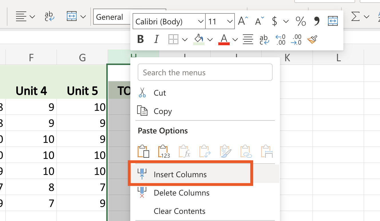
• New Rows, New Columns: You can insert a new row directly below or above the row number where you want it to appear. To add a new row, right-click the row label immediately below where the insertion should occur, then select ‘Insert’. You can add a new column immediately to the left or right of the column letter where it should appear. To add a new column, right-click the column letter immediately to the left or right of the point where it should appear, then select ‘Insert’. This action will shift existing rows or columns one space to the right, allowing you to insert a new row or column where needed.

•  Clean Up Your Spreadsheet: If you find a row you don’t need, right-click on the row number—in this case, F:9—and select ‘Delete’. For columns, the process is the same, except you right-click on the column letter. This will visually highlight the selected range on your screen so you can confirm what you’re deleting.

Hiding and Unhiding Rows and Columns

•  Hide Rows and Columns to Visualise Your Data More Clearly: To hide rows, right-click the row number and deselect ‘Show’. To hide columns, right-click the column letter and deselect ‘Show’. This action hides the cells while preserving the data in the background, allowing you to unhide the cells later if needed.

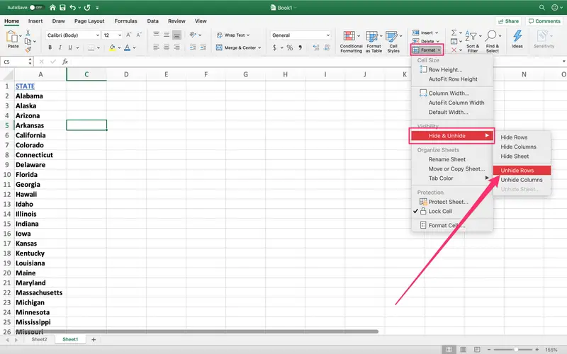
•  Unhiding Rows and Columns to Reveal Hidden Data: To unhide rows or columns, click on the row above or column to the left of the hidden row or column. Right-click and choose ‘Unhide’. The hidden data will now be revealed. You can then edit the data as usual. Always unhide the data when you want to resume working on something that’s been out of sight, for quicker data organisation purposes.

Adjusting Row Height and Column Width

• Better Readability by Changing Size of Rows and Columns to Fit Data: Change the size of rows and columns for better readability. To do this, ensure you have the row numbers at the left of the row headings or the column letters at the top of the column headings visible. Move your cursor over the boundary between the row numbers or column letters (so that it turns into a double-headed arrow; see Figure 4 below). Then click and drag to make the rows or columns bigger (or smaller) so that the data fits perfectly between cells.

•  Auto-Fitting the Size of Rows and Columns: The size of rows and columns in Excel Online can dynamically adjust to fit the content of the cells they contain. To manually adjust the size of any row or column, simply double-click the border separating the numbered rows or lettered columns, and the size of said row or column will resize dynamically to the smallest appropriate size encompassing all the data in the row or column, respectively.

Using Formulas and Functions in Microsoft Excel Online

Using Formulas and Functions in Microsoft Excel Online empowers users to perform complex calculations and automate data processing effortlessly. Formulas, such as SUM, AVERAGE, and COUNT, enable quick aggregation and analysis of data, while functions like IF, VLOOKUP, and CONCATENATE enhance data manipulation and decision-making. Whether managing budgets, analysing trends, or organising information, Excel Online provides powerful tools to streamline tasks and maximise productivity in a collaborative online environment.

Basic Formulas

• Excel Online supports basic arithmetic operations: Plus (+), minus (-), an asterisk (*), and forward slash (/). These operations perform calculations based on the data entered into your spreadsheet. For instance, to add values from two cells, you can use a formula like A1+B1.

•  Building Basic Formulas for Calculations: To build a formula, simply open a cell, press the equal sign (‘=’), and then enter an arithmetic operation. For instance, =A1*B1 multiplies the values in cells A1 and B1. Formulas can reference specific cells, allowing you to calculate your database values and update them automatically whenever data changes.

Common Functions

• Aggregate Functions (SUM, AVERAGE, and COUNT): Excel provides functions such as SUM, AVERAGE, and COUNT, which help simplify complex calculations. For example, the SUM function adds up a range of cells (e.g., =SUM(A1)), while AVERAGE calculates the mean of a range (e.g., =AVERAGE(B1)). The COUNT function counts the number of numeric entries in a range (e.g., =COUNT(C1)). These functions are essential for basic data analysis.

•  Logical Functions (IF, AND, OR): You will use logical functions to perform conditional calculations. For example, the IF function performs a calculation if a specific condition is met (=IF(A1>10, “High”, “Low”)): =IF(A1>10, “High”, “Low”). When you need a cell’s value to change only if multiple conditions are met, use the AND function, like this: =AND(A1>10, B1<5): =AND(A1>10, B1<5). Alternatively, if you want a cell’s value to change if at least one condition is met, use the OR function: =OR(A1>10, B1<5)OR(A1>10, B1<5).

Copying Formulas Using Relative and Absolute References

•  Relative vs absolute References: When you copy a formula, the reference changes based on whether it’s relative (e.g. A1) or absolute (e.g. $A$1). A relative reference adjusts based on where the formula is pasted relative to its original location. In contrast, an absolute reference ($A$1) remains unchanged regardless of where the formula is pasted. Understanding this distinction is crucial to maintaining the accuracy of your formulas.

•  Copying Formulas Across Several Cells Correctly: To copy a formula from one cell to others, select the cell containing the formula, then drag the fill handle (a small square at the bottom-right corner of the cell) to the last cell where you want to copy it. Excel will automatically replicate the relative references for you. If you need to keep a reference fixed, use absolute references by adding dollar signs ($) before the column letter and row number in your cell reference.

Enroll in our Microsoft Excel Course

Data Validation and Error Checking in Microsoft Excel Online

Data Validation and Error Checking are essential features in Microsoft Excel Online, ensuring data accuracy and reliability. Data Validation allows users to control what can be entered into a cell by setting criteria such as number ranges, dates, text length, and more. This helps maintain consistency and prevents errors in data entry.

Error Checking, on the other hand, identifies and highlights common errors in formulas or data entries, such as incorrect cell references, circular references, and potential calculation errors. It provides suggestions and options to correct these errors, ensuring the accuracy of your calculations and analyses.

Together, these tools enhance data quality, streamline workflow efficiency, and minimise the risk of mistakes in Excel Online.

Setting Up Data Validation Rules

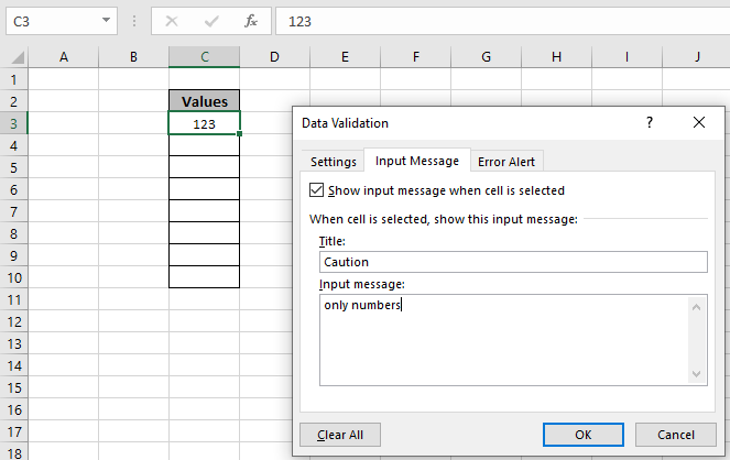
•  Validation Rules for Accuracy: Data validation rules in Office Excel Online help ensure data accuracy by controlling the data-entry process. To set up data validation, select the cells where you want the rules, then navigate to Home > Data > Data Validation. You can define criteria to limit the type of data that can be entered into these cells. For example, you can restrict entries to whole numbers, decimal values, a range of dates, values from a list, or dates between two specified dates. Setting up data validation may seem intimidating, but it’s straightforward. You can make it as simple or as complex as needed. By applying these rules, any errors entered as data will be flagged, reducing mistakes and ensuring data integrity.

•  Standardise data using drop-down lists for consistency: Standardising and checking data as it is entered is essential. One way to do this is by using drop-down lists. To create a drop-down list, select the cells, click on the ‘Data’ tab, then ‘Data Validation’. Stay on the ‘Settings’ tab and choose ‘List’. Enter the permissible values into the box, separated by commas. This will create a drop-down list next to each cell, allowing you to select the desired value. You can use this method to categorise and standardise your data, ensuring users select only from specific options.

Identifying and Correcting Errors

• Catching Mistakes with Error-Checking Tools:Excel Online includes several tools to help you identify and manage data errors. For instance, if you attempt to divide by zero in a formula or reference an invalid cell lacking data, Excel displays a small green triangle in the top-left corner of the affected cell. Clicking this triangle provides various options to correct or ignore the error. Regularly using these tools ensures your data remains error-free.

•  Avoid common data entry errors in cells and formula mistakes: Common data entry mistakes and formula errors can be easily rectified with a few simple steps. For a data entry error, simply double-click on the cell containing the mistake to edit its content. For formula errors, Excel usually provides error hints, such as referencing an empty cell. Here’s what you can do:
  1. Identify the source of the mistake.
  2. For simple formula errors, correct them immediately.
  3. Use ‘Trace Error’ from the error checking menu to pinpoint and visualize the source of the mistake, making it easier to make the necessary adjustments to the formula.

Collaboration Features in Microsoft Excel Online

Microsoft Excel Online offers comprehensive collaboration features that allow multiple users to work on spreadsheets simultaneously from different locations. Users can view changes in real-time, facilitating seamless and efficient collaboration. Features include real-time co-authoring, where multiple users can edit a spreadsheet concurrently. Comments and chat functionalities enable easy communication and feedback exchange directly within the Excel Online interface. These collaborative tools enhance productivity and teamwork, making it easier to collaborate on complex projects or shared datasets.

Sharing and Co-Authoring Workbooks

•  Share your Excel Online workbooks for collaboration: People can easily collaborate when sharing workbooks in Excel Online. Look at the top-right corner of your screen and click the Share button. Enter the email addresses of your collaborators, choose their permissions (view or edit), and optionally add a message. Alternatively, share your file using a link that you can send directly to your collaborators. This ensures everyone uses the same version and has access to the updated file.

•  Co-Authoring feature to make it easier to work in real-time: Co-authoring is a collaborative feature of Excel Online that allows colleagues to create workbooks simultaneously. Any changes made by authors are reflected in real-time, and you can see which section of the document others are working on concurrently. This feature simplifies real-time collaboration, reducing the risk of discrepancies in updated workbooks. Co-authoring is particularly effective for team-based projects involving multiple stakeholders, ensuring everyone works on the same version and avoiding versioning conflicts. For instance, in an Excel file for a team budget involving more than five colleagues, managers can gather input from various departments to allocate budgets for the new year.

Commenting and Reviewing Changes

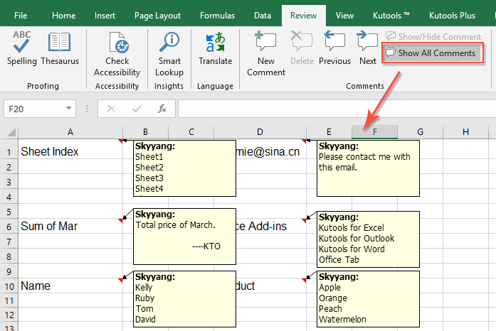
•  Adding And Managing Comments To Provide Feedback: You can gather feedback from colleagues on your data points by adding and managing comments in Excel Online. Simply right-click on any cell, select “New Comment” from the menu, and a comment popup will appear. Type your feedback and press Enter to post it. To reply to a comment and create a thread, click on the comment and type your reply. Comments not only serve as feedback but also facilitate discussions and decisions on complex points within your workbook.

•  Track changes and review collaboration updates: In Microsoft Excel Online, you can track changes and review collaboration updates. Use the ‘Track Changes’ tool located under the Review tab to see modifications made by others. Different users are identified in Excel cells that have been altered, allowing you to review and edit the changes. You can also accept or reject updates made by others, giving you control over your document’s final version.

Advanced Editing Techniques in Microsoft Excel Online

Advanced Editing Techniques in Microsoft Excel Online include a variety of powerful tools and methods to refine and manipulate data efficiently. These techniques cover complex formula editing, advanced data sorting and filtering, custom formatting, pivot tables for dynamic data analysis, and collaboration features like co-authoring and version control. Mastering these tools allows users to manage and present data with precision and clarity, enhancing productivity and decision-making capabilities in professional environments.

Using Find and Replace

•  Find and Replace: Excel Online allows you to quickly find and replace specific data in any worksheet. To find data, type the text or number you want to locate in the selected data and press Ctrl+F. This will open the Find dialog box where you can search for the entered text or number within the cells. For replacing specific data, press Ctrl+H to open the Replace dialog box. Enter the text you wish to find in the ‘Find what’ text box and the replacement text in the ‘Replace with’ box. Click ‘Replace All’ to update all instances or ‘Replace’ to update them one by one.

•  Enhanced Find And Replace Command: Looking for a more sophisticated way to edit a spreadsheet? For faster editing, utilize the enhanced Find and Replace command in Excel Online. Click on ‘Options’ within the Find or Replace dialogue box to access these settings. Here, you’ll find additional options such as matching cases, searching within specific sheets or workbooks, or limiting searches to cell contents only. This function empowers you to edit spreadsheets effectively, ensuring accuracy without errors.

Freezing Panes and Splitting Windows

•  Maintaining Visibility of Headers through Freeze Panes: Useful for displaying row and column headers throughout a large dataset, the Freeze Panes feature in Excel retains headers while scrolling through data, typically the largest portion of a sheet. Found under the View tab, click on ‘Freeze Panes’ and select either ‘Freeze Top Row’, ‘Freeze First Column’, or ‘Freeze Panes’ based on your needs. This simple tip enhances readability by preserving context and improves efficiency when conducting detailed analytical work with data.

•  Split windows to view multiple workbook sections at once: Perform a window split to view two different parts of the workbook simultaneously. Open the View tab, click Split to divide the window. Move the cursor over a divider until it becomes a double-headed arrow, then drag it to where you want. Add more splits as needed. Once done, rejoin the splits to compare information side by side. This is especially useful for large spreadsheets to avoid frequent scrolling.

Using Data Filters

•  Using Filters to Analyse Data in Excel Online: Filters in Excel Online allow you to view subsets of your data based on specific categories or conditions. To apply a filter, first select the range of cells you want to filter. Then, navigate to the Data tab and click on Filter. An Arrange box will appear, allowing you to choose the range of cells to filter. Once selected, the Arrange box will display a Show button. Clicking on this button creates an empty rectangle that hides all data except the subset you want to focus on. To complete the process, click ‘Select all’ and then ‘OK’. Next, click the arrow on the right side of each header to choose filter criteria (e.g., values or conditions) that highlight the relevant subset of your data.

•  Filter Criteria for Targeted Data Views: Excel Online allows you to customise filter criteria to achieve highly targeted views of your data. After selecting the cell, column, or table to filter, you can specify criteria such as ‘equals’, ‘contains’, ‘greater than’, or ‘between’. These custom filters enable you to retrieve the most specific and relevant data records for in-depth analysis and informed decision-making.

Conclusion

Whether you are a beginner or an experienced data editor, you will find all the essential functions for data entry, formatting, editing, advanced tools, Power Query, and collaboration features available online. Using these tools enables you to manage and edit data more efficiently, enhancing teamwork effectively. With Excel Online as your data management system, you can practise all functions whenever and wherever you need.